Get Pedestrian Frequency Data from the Hystreet Project • hystReet

Introduction

hystreet is a company that collects data on pedestrian traffic in shopping streets of different German cities. After registering you can access and download the data via their website.

Installation

The package is now on CRAN. The easiest way to download is via:

install.packages("hystReet")

You can install the development version from GitHub with the following command:

if (!require("devtools"))
  install.packages("devtools")
devtools::install_github("JohannesFriedrich/hystReet")

API Keys

To use this package, you will first need to get a hystreet API key. To do so, you first need to set up an account on https://hystreet.com/. After that you can request an API key via e-mail. Once your request has been granted, you will find you key in your hystreet account profile.

Now you have three options:

Once you have your key, you can save it as an environment variable for the current session by running the following command:

Sys.setenv(HYSTREET_API_TOKEN = "PASTE YOUR API TOKEN HERE")

Alternatively, you can set it permanently with the help of usethis::edit_r_environ() by adding the following line to your .Renviron:

HYSTREET_API_TOKEN = PASTE YOUR API TOKEN HERE

If you don’t want to save your API token here, you can enter it for each function of this package using the API_token parameter.

Usage

Function name	Description	Example
get_hystreet_stats()	request common statistics about the hystreet project	get_hystreet_stats()
get_hystreet_locations()	request all available locations	get_hystreet_locations()
get_hystreet_station_data()	request data from a stations	get_hystreet_station_data(71)
set_hystreet_token()	set your API token	set_hystreet_token(123456789)

Load some statistics

The function get_hystreet_stats() summarises the number of available stations and the sum of all counted pedestrians.

library(hystReet)
## Loading required package: httr
## Loading required package: jsonlite
## 
## Attaching package: 'jsonlite'
## The following object is masked from 'package:purrr':
## 
##     flatten

stats <- get_hystreet_stats()

stats

stations	today_count
188	2260884

Request all stations

The function get_hystreet_locations() generates a data frame with all available stations of the project.

locations <- get_hystreet_locations()

locations

id	name	city
308	Leipziger Straße (West)	Halle (Saale)
76	Königstraße (Mitte)	Stuttgart
351	Johann-Philipp-Straße	Trier
108	Große Straße (Mitte)	Osnabrück
309	Hochstraße (Nord)	Krefeld
140	Fleischstraße (Nord)	Trier
53	Schadowstraße (West)	Düsseldorf
55	Flinger Straße (Ost)	Düsseldorf
348	Holstenstraße (Nord)	Kiel
368	Marktstraße	Mönchengladbach

Request data from a specific station

The (probably) most interesting function is get_hystreet_station_data(). Using the hystreetID it is possible to request a specific station. By default, all the data from the current day are received. With the query argument it is possible to define the time and sampling frame of the data more precisely:

from: datetime of earliest measurement (default: today 00:00:00:): e.g. “2021-10-01 12:00:00” or “2021-10-01”
to : datetime of latest measurement (default: today 23:59:59): e.g. “2021-12-01 12:00:00” or “2021-12-01”
resoution: Resolution for the measurement (default: hour): “day”, “hour”, “month”, “week”

data <- get_hystreet_station_data(
  hystreetId = 71,
  query = list(from = "2021-12-01", to = "2021-12-31", resolution = "day"))

Some ideas for visualising the data

Let´s see if we can find the busiest days in December 2021. Saturdays were probably quite busy, while there should have been substantially less pedestrian traffic on the 25th and 26th of December, both of which are holidays in Germany.

data <- get_hystreet_station_data(
    hystreetId = 71, 
    query = list(from = "2021-12-01", to = "2022-01-01", resolution = "hour"))

ggplot(data$measurements, aes(x = timestamp, y = pedestrians_count, colour = weekdays(timestamp))) +
  geom_path(group = 1) +
  scale_x_datetime(date_breaks = "7 days", labels = date_format("%d.%m.%Y")) +
  labs(x = "Date",
       y = "Pedestrians",
       colour = "Day")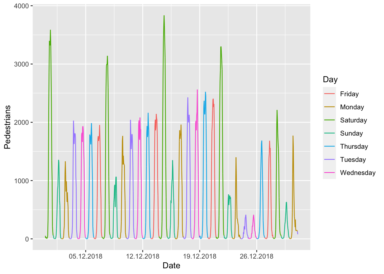

Compare different stations

Now let´s compare data from different stations:

Load the data

data_73 <- get_hystreet_station_data(
    hystreetId = 73, 
    query = list(from = "2022-01-01", to = "2022-01-31", resolution = "day"))$measurements %>% 
  select(pedestrians_count, timestamp) %>% 
  mutate(station = 73)

data_74 <- get_hystreet_station_data(
    hystreetId = 74, 
    query = list(from = "2022-01-01", to = "2022-01-31", resolution = "day"))$measurements %>% 
    select(pedestrians_count, timestamp) %>% 
  mutate(station = 74)

data_73_74 <- bind_rows(data_73, data_74)

ggplot(data_73_74, aes(x = timestamp, y = pedestrians_count, fill = weekdays(timestamp))) +
  geom_bar(stat = "identity") +
  scale_x_datetime(labels = date_format("%d.%m.%Y")) +
  facet_wrap(~station, scales = "free_y") +
  theme(legend.position = "bottom",
        axis.text.x = element_text(angle = 45, hjust = 1))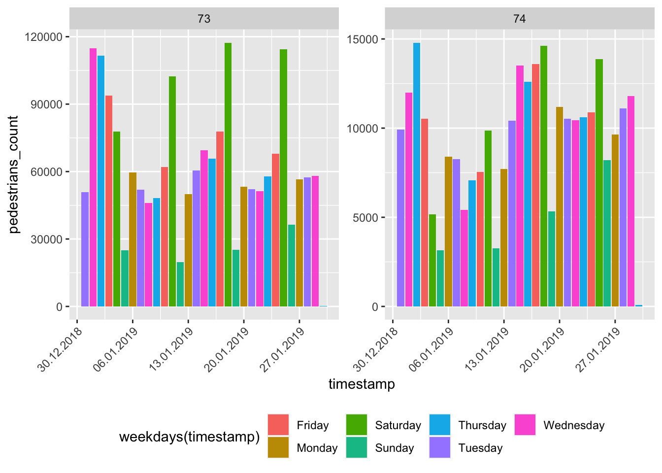

Highest ratio (pedestrians/day)

Now a little bit of big data analysis. Let´s find the station with the highest pedestrians per day ratio:

hystreet_ids <- get_hystreet_locations()

all_data <- lapply(hystreet_ids[,"id"], function(ID){
  temp <- get_hystreet_station_data(
    hystreetId = ID,
    query = list(from = "2021-01-01", to = "2021-12-31", resolution = "day"))
  
  
    lifetime_count <- temp$statistics$timerange_count
    days_counted <- as.integer(ymd(temp$metadata$measured_to)  - ymd(temp$metadata$measured_from))
    
    return(data.frame(
      id = ID,
      station = paste0(temp$city, " (",temp$name,")"),
      ratio = lifetime_count/days_counted))
  
})

ratio <- bind_rows(all_data)

Which stations have the highest ratio?

ratio %>% 
  top_n(5, ratio) %>% 
  arrange(desc(ratio))
##    id                           station    ratio
## 1  73  München (Neuhauser Straße (Ost)) 45510.15
## 2 165         München (Kaufingerstraße) 42458.42
## 3 305    Wien (Kärntner Straße (Mitte)) 40067.34
## 4 306 Wien (Mariahilfer Straße (Mitte)) 39642.14
## 5  63            Hannover (Georgstraße) 38442.91

Now let´s visualise the top 10 locations:

ggplot(ratio %>% 
         top_n(10,ratio), aes(station, ratio)) +
  geom_bar(stat = "identity") +
  labs(x = "Location",
       y = "Pedestrians per day") + 
    theme(legend.position = "bottom",
        axis.text.x = element_text(angle = 45, hjust = 1))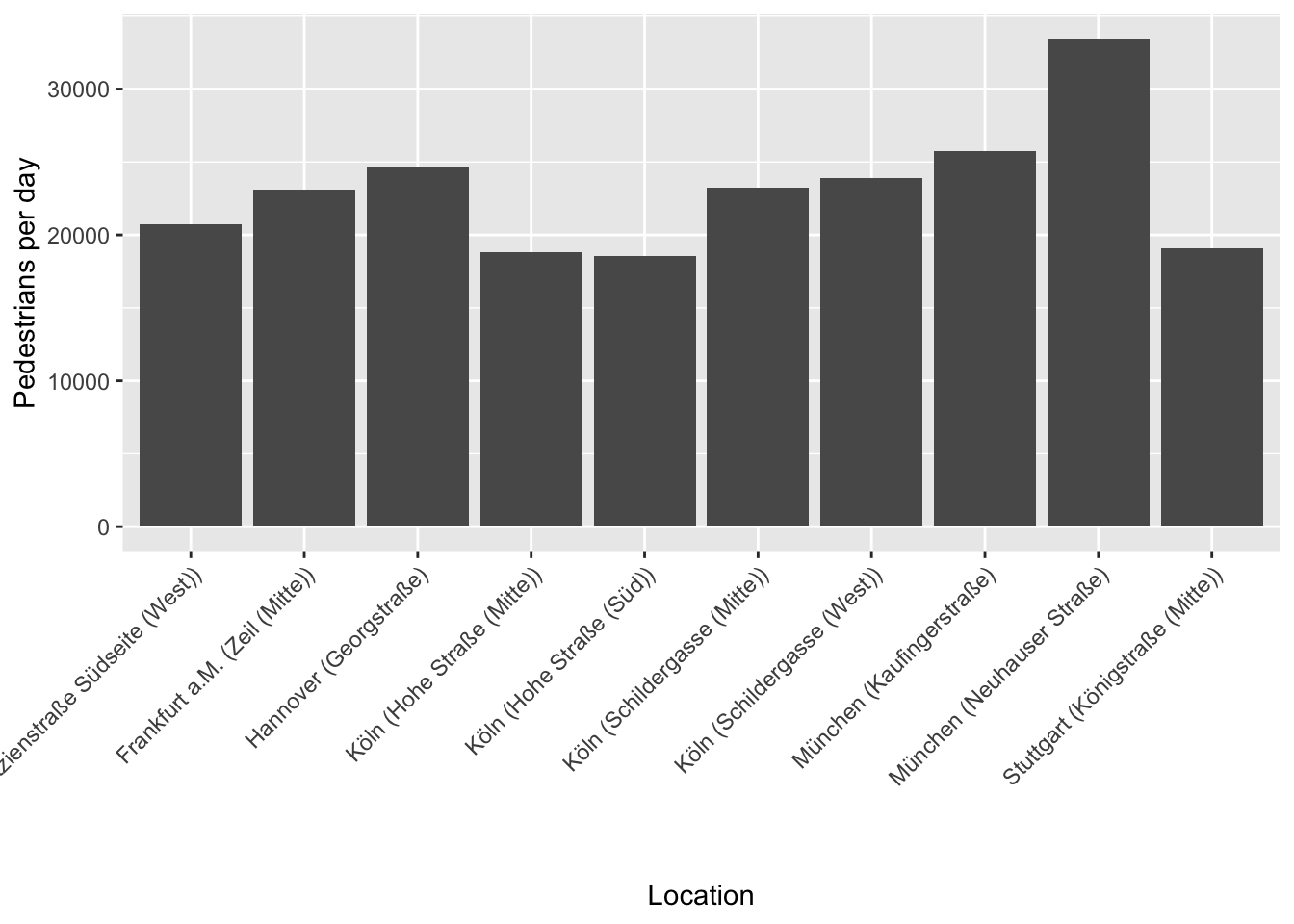

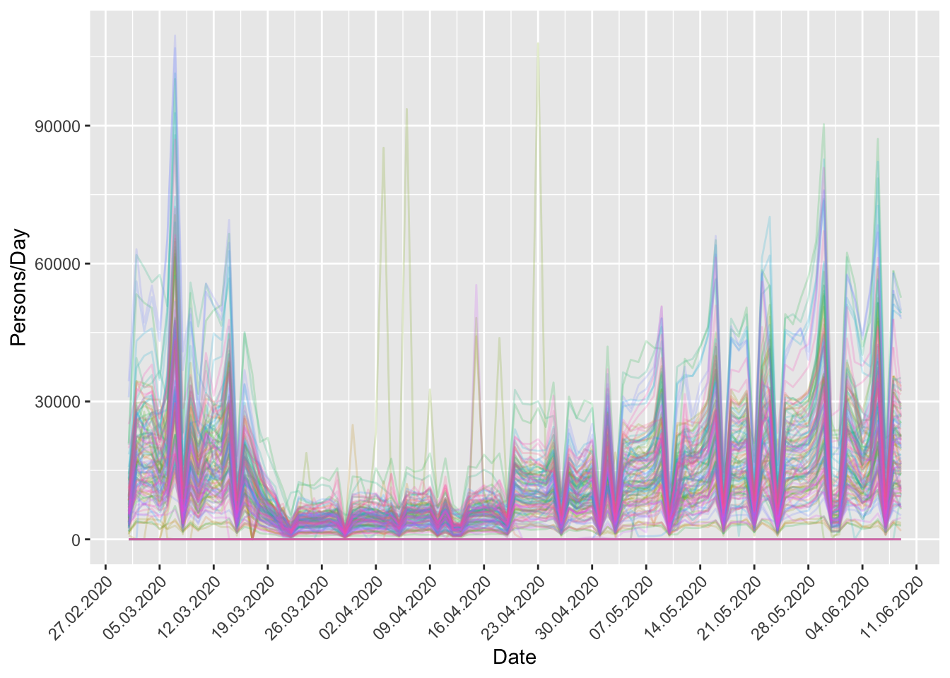
Corona effects

The Hystreet-API is a great source of analysing the social effects of the Corona pandemic in 2020. Let´s collect all german stations since March 2020 and analyse the pedestrian count until 10th June 2020.

data <- lapply(hystreet_ids[,"id"], function(ID){

    temp <- get_hystreet_station_data(
        hystreetId = ID,
        query = list(from = "2020-03-01", to = "2020-06-10", resolution = "day")
    )
    
    return(data.frame(
    name = temp$name,
    city = temp$city,
    timestamp = format(as.POSIXct(temp$measurements$timestamp), "%Y-%m-%d"),
    pedestrians_count = temp$measurements$pedestrians_count,
    legend = paste(temp$city, temp$name, sep = " - ")
  ))
   
}) 

data_all <- bind_rows(data)

data_all %>% 
ggplot(aes(ymd(timestamp), pedestrians_count, colour = legend)) +
geom_line(alpha = 0.2) +
    scale_x_date(labels = date_format("%d.%m.%Y"),
               breaks = date_breaks("7 days")
     ) +
  theme(legend.position = "none",
        legend.title = element_text("Legende"),
         axis.text.x = element_text(angle = 45, hjust = 1)) +
  labs(x = "Date",
       y = "Persons/Day")